Quantifying Prediction Difficulty

I’ve been working on uncertainty quantification for deep learning models. Most recently, I collaborated on the paper Decision-Focused Uncertainty Quantification, where we explored ways to extend the standard conformal prediction method to generate more useful prediction sets for decision-makers.

As part of the project, we needed to quantify the difficulty of classifying an image using a specific model and connect that difficulty to the set size that resulted from conformal prediction. More specifically, we wanted to prove that difficult images resulted in larger predicted sets. This post discusses the two methods we considered for measuring prediction difficulty and why we chose one over the other.

Entropy of the Softmax Distribution

The intuition behind this method is to leverage the shape of the softmax distribution to determine the certainty of the model’s prediction. If the model is sure about its prediction, the output softmax distribution will have a dominant class with a score of around 0.99, while the other classes will have tiny scores. If the model is unsure which class to assign the image to, the softmax distribution will be mostly flat—i.e., all images will have roughly the same score.

As a former physicist, I can’t help but think of the entropy as a measurement of the flatness of the softmax distribution. We are going to use Shannon’s entropy in the context of information theory, which is given by

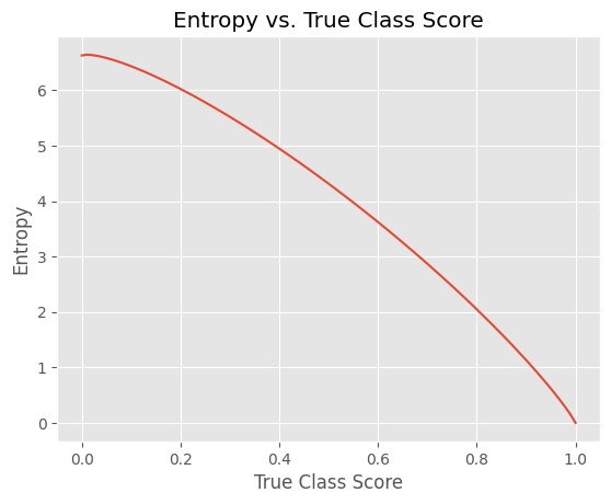
The entropy of the softmax distribution will be large if we have a flat distribution because it’s the state of largest uncertainty. In that case, the flat distribution resembles a uniform distribution where we really don’t know which class we should assign to the image.

In contrast, the entropy of the softmax output will be small if we have a peak in one of the classes. Intuitively, this will be where we have less uncertainty about our prediction. Mathematically, we can use the entropy equation to analyze why the entropy will be small. The class that has the peak \(p_k \sim 1\) and \(\log(p_k) \sim 0\). For all the other classes, \(p_k \sim 0\). That means all the terms on the sum in the entropy equation will be small.

We can verify this with a toy example where we vary the score of one of the classes and distribute the remaining density across the other classes. The snippet below does exactly that and produces the plot we expect.

import matplotlib.pyplot as plt
import numpy as np

from scipy import stats

true_class_scores = np.linspace(0, 1, 100)
n_classes = 100
entropies = []

for true_class_score in true_class_scores:
    extra_class_score = (1 - true_class_score) / (n_classes - 1)
    extra_classes = [extra_class_score] * (n_classes - 1)
    softmax_output = np.array(
        [true_class_score] + extra_classes
    )
    entropies.append(stats.entropy(softmax_output, base=2))

Score of the True Class

This is a short description because the method is pretty simple. Another way to quantify the difficulty of an image for a model is to quantify the model’s expected accuracy. This calculation is easier because we can just use the true label’s softmax score to measure the model’s expected accuracy for a specific image. The score will not be perfectly calibrated to a probability, but it will be good enough to measure difficulty. If the softmax score is small for the true class, the probability of the model being right for that image is also small.

The Verdict

We ended up using the score of the true class for the following reasons related to how conformal prediction impacts the predicted set:

1. Conformal prediction, by definition, will output a larger set if the distribution is flatter because we need more classes to reach the conformal score threshold. That means the “flatness” of the distribution is not a good metric because the relationship between difficulty and set size is pre-defined—i.e., we can’t have difficult examples with small sets.

2. The score of the true class ignores the score of the other classes. If the true class has a low score, it doesn’t necessarily mean the set will be large because other classes may have large scores that reach the threshold with just a few classes. In other words, we could have a small set size and a model that assigns a high score to the wrong class. That means the example is difficult to classify because it confuses the model and has a small set size. Since our objective was to prove that our method had large sets for difficult images, this difficulty definition was perfect for us.

I really enjoyed thinking about this problem because both methods are good ways to quantify the model’s uncertainty. However, in conformal prediction, we have a clear winner when determining the effect of prediction difficulty on the set size.