Initializing the Bias in Output Layers
One of Andrej Karpathy’s recommendations in his famous A Recipe for Training Neural Networks is to “initialize well.”
If you have an imbalanced dataset of a ratio 1:10 of positives:negatives, set the bias on your logits such that your network predicts probability of 0.1 at initialization. Setting these correctly will speed up convergence and eliminate “hockey stick” loss curves where in the first few iteration your network is basically just learning the bias.
I have used his advice to initialize my binary classifiers and, so far, have achieved good results. However, I never stopped to test whether initializing the bias with that recommendation helped model performance significantly. This post aims to answer that question with a quick experiment.
The Setup
-
Dataset: We are going to use the CIFAR10 dataset with a twist. The twist is that we want to benchmark the bias initialization in a binary task, but CIFAR10 has ten classes. We will follow the Hot Dog-Not Hot Dog approach to turn the task into a binary classification problem. We don’t have hot dogs in CIFAR10, so we will train a model that classifies Frog-Not Frog.
-
Model: We used EfficientNet B1 with ~7.8M parameters available in torchvision. This model strikes a good balance between speed and performance: it is small enough to run multiple experiments quickly but performs well, as measured by its acc@1 of 79.838 on ImageNet. We ran experiments with and without pre-trained ImageNet weights to check whether the pre-training impacted our results.
-
Training: We trained each model for five epochs and repeated each training process ten times to account for randomness in initialization and training. The optimizer is the vanilla SGD with a learning rate of 0.0001. You can see all the training details in this GitHub link.
-
Hardware: We ran the experiments in a T4 GPU, which is right for this experiment because the model and the data aren’t too large. Training the two models ten times each costs less than USD 10 on a single T4. I ran everything using Lightning Studios, which has proven great for quickly spinning up instances with GPUs and running experiments.
Results
ImageNet Weights
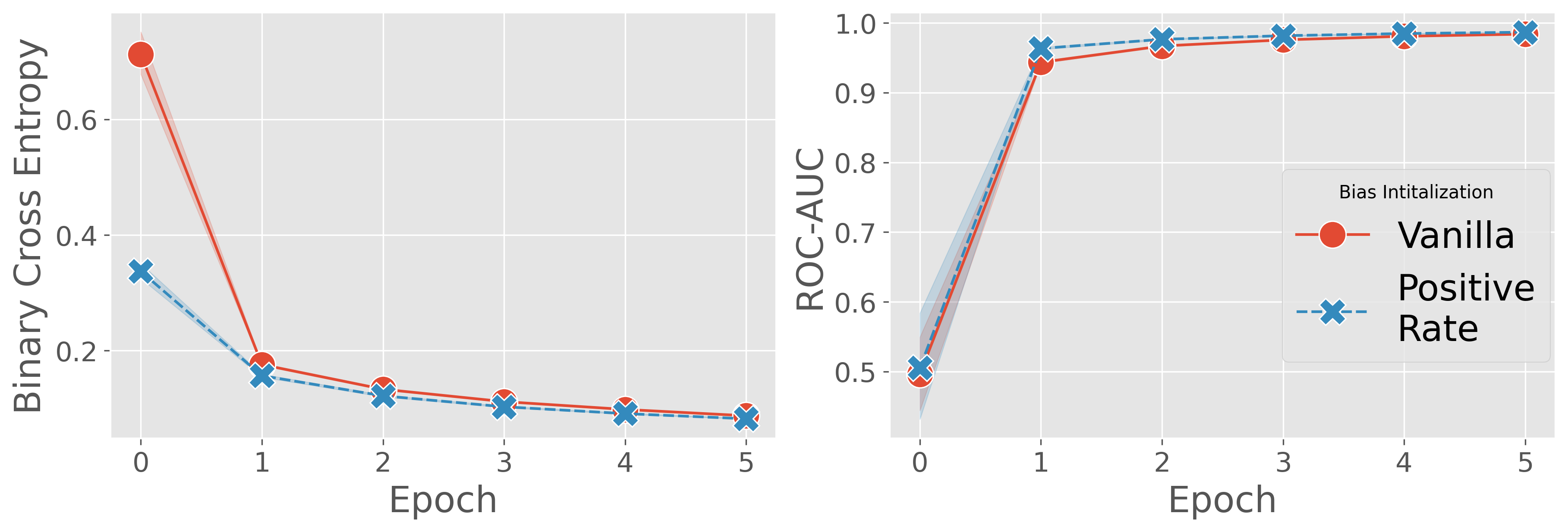
The first experiment was to train the model using the pre-trained ImageNet weights. The learning curve at epoch 0 shows how initializing the model at the positive class rate starts with a lower loss before training the model. However, the model with the vanilla initialization quickly closes the gap, and both models have identical performance by the 5th training epoch.
Despite both models achieving nearly identical performance after a few epochs, the positive rate initialization avoids the hockey stick shape in the learning curve. This head start in the loss may be crucial for larger datasets or models you can’t afford to train for multiple epochs.

Trained without ImageNet Weights
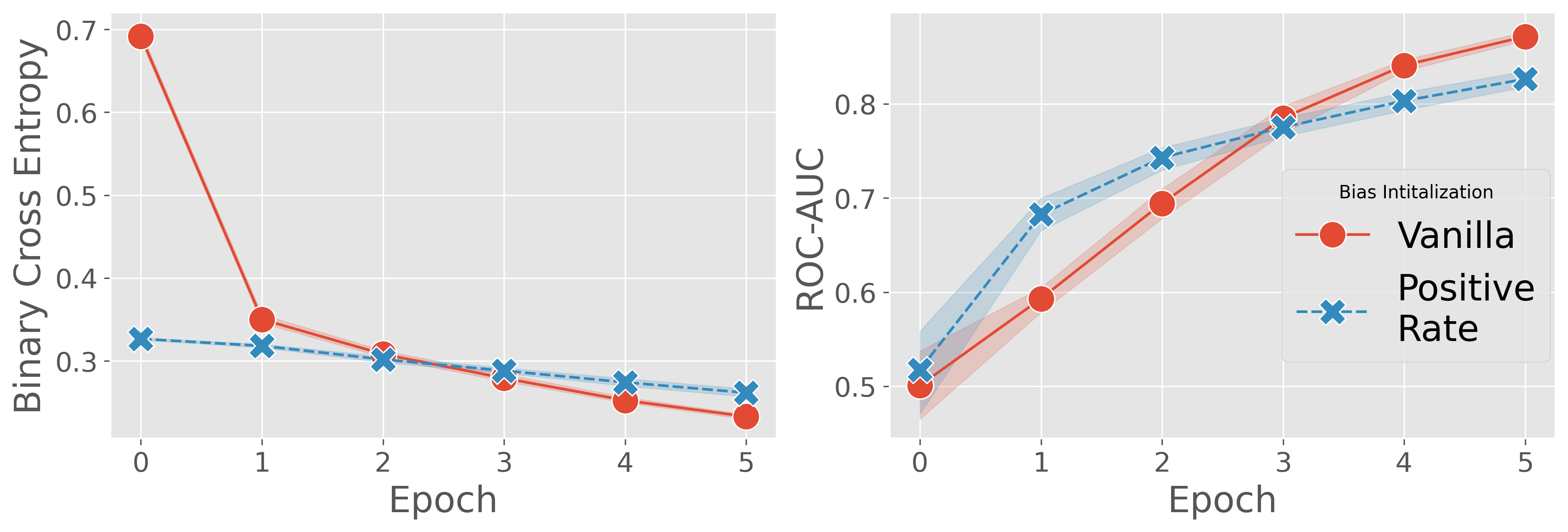
The second experiment was to train the model without the pre-trained ImageNet weights. The first—perhaps expected—conclusion is that we have a harder time training the model without the ImageNet weights. Both initializations achieved less than 0.9 ROC-AUC in the fifth epoch, while the model with ImageNet weights was already close to perfect ROC-AUC at that point in training.
As before, the positive rate initialization has a head start from the model initialized with the vanilla output bias. If we focus on the ROC-AUC learning curve, the red curve has a harder time catching up with the blue curve up to the third epoch. This indicates that the advantage given by the positive rate initialization is more valuable in the case of models without pre-trained weights.
What’s interesting about the plot below is how the vanilla initialization model surpasses the positive rate initialization model. None of the two models have converged, but you would benefit from choosing the vanilla initialization if your FLOPs budget only allowed for training five epochs.

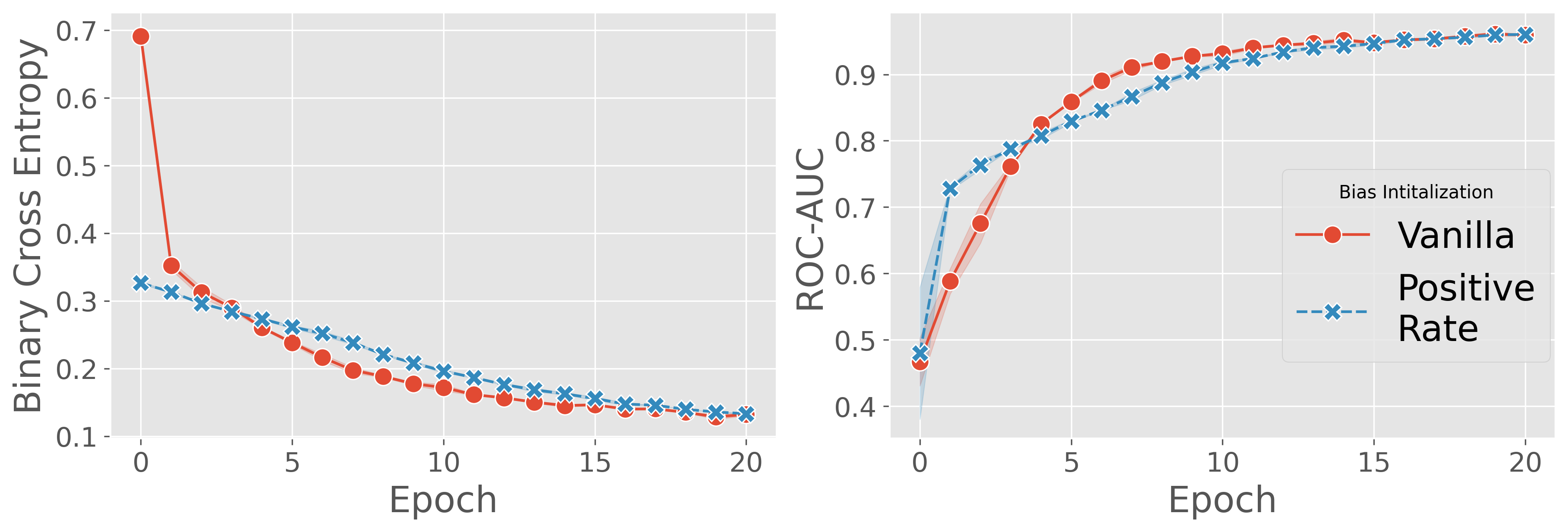
To compare the model with the pre-trained weights, we trained both models without the ImageNet weights until they converged. The plots below are just from training the models twice instead of ten as from the previous two plots.
The conclusion is the same as with the ImageNet weights: both models achieve similar metrics if we can afford to train them to convergence.

Takeaways
Initializing the bias in the model’s output layer with the positive class rate, as Karpathy mentions in his guide, avoids the hockey stick shape in the learning curve. This head start proves useful when your FLOPs budget can only afford a few training epochs. However, the model initialized with the vanilla method closes the gap quickly for the pre-trained model and after a few epochs for the model trained from scratch.
Also, always use pre-trained weights when possible! The strongest conclusion from this set of runs is that models with pre-trained weights converge significantly faster than models trained from scratch.