Mean vs. Total Cross-Entropy Loss
I recently started my MSc in Artificial Intelligence at the University of Amsterdam, so I am reviewing deep learning fundamentals. Those fundamentals include using pure Numpy to write the components of a neural network and use them to train a simple model on CIFAR10 with linear layers and ELU activations. The dataset has 10 classes, so using the softmax function in the last layer and the cross-entropy as the loss function is natural.
I started implementing the forward and backward passes, feeling lucky to have frameworks like PyTorch and JAX that save us from implementing these parts (especially the backward pass) when using neural networks. Everything looked good with the forward and backward passes, so it was time to move on to training the neural network.
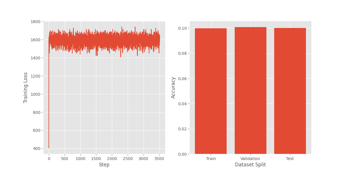
Fortunately, the training loop ran quickly and got the first results in a few minutes. Unfortunately, they looked like this:

There was something clearly wrong with the model, and since I wasn’t standing on the shoulders of PyTorch or JAX, I wasn’t sure where to begin to debug.
My first instinct was to implement the model in PyTorch and check layer by layer to see if I was getting the same result as my Numpy implementation. This wasn’t fun. I had to initialize the numpy and PyTorch networks to the same values and make the layer values reproducible. After hours of checking tensors and arrays of outputs and gradients, I convinced myself that the layer implementations had identical results.
Could it be something with the initialization? I was getting warnings about potential overflows and wondered if my implementation of the Kaiming initialization was causing large values and exploding the values and gradients of the network. I tried multiple initialization methods and was still getting the same curve.
It was getting dark outside, so I returned to the pipeline I had replicated in PyTorch and began reading the parameters of each of the layers. I had defaulted to using the sum reduction for the cross-entropy
-np.sum(y_ohe * np.log(x + 1e-6))
which in PyTorch is equivalent to
nn.CrossEntropyLoss(reduction=”sum”)
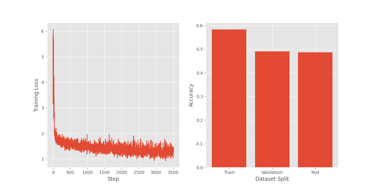
I realized I was using a parameter different from PyTorch’s default. Changing to the default mean reduction resulted in the plot below. Beautiful.

I then changed my numpy implementation of the cross entropy loss and got the same nice (and expected!) curve above. The implementation now looked like this
(1 / y.shape[0]) * -np.sum(y_ohe * np.log(x + 1e-6))
A small but very consequential change! It basically was the difference between a usable and unusable model, and it is a mistake I could have also made in PyTorch by setting the wrong parameter value.
In retrospect, I should have remembered that using the sum of the loss function brings problems:
-
Training instability if the batch size is large because the gradient—and therefore the parameter update—becomes large. This is true, especially if you haven’t tuned your learning rate.
-
You can’t easily compare losses between runs if you change the batch size between them.
Number 1 was the cause of my problems this time, but number 2 was problematic when running multiple experiments.
So, as a reminder to my future self, use the mean loss function unless there is a good reason not to!